Week 7 (June 27 - July 1, 2022)
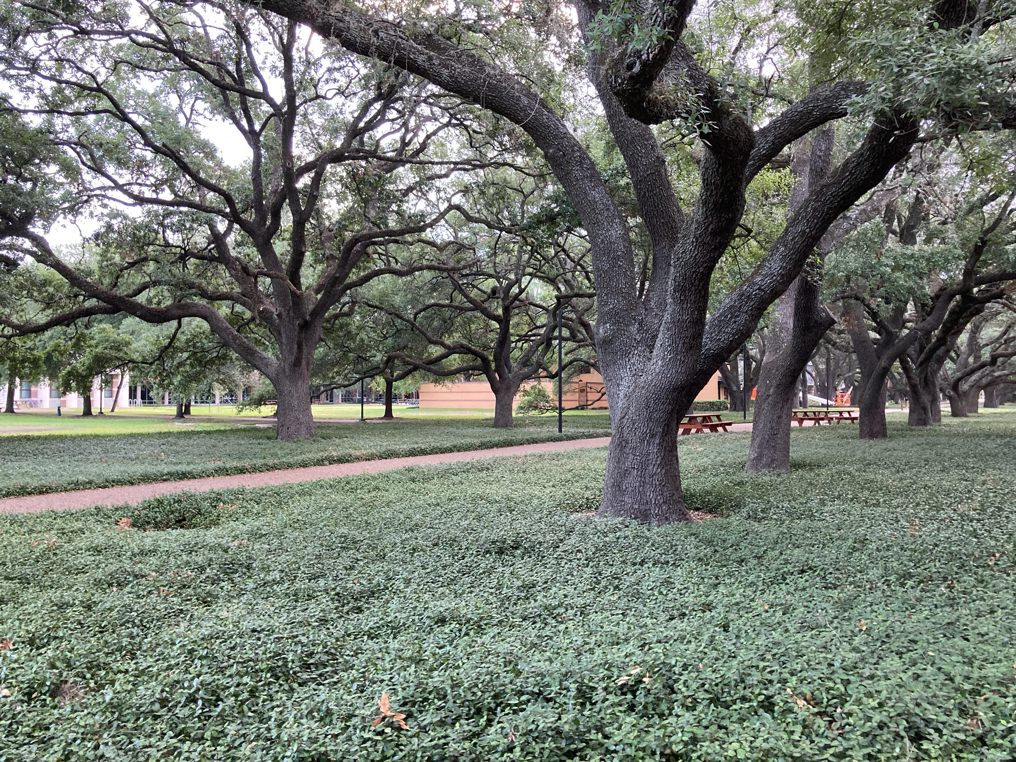
This week I finally flew to Rice and began in-person work. It has been nice exploring campus the past few days and meeting Professor Ordóñez-Román, Ziyan, and Veronica. Rice’s campus is very different from Columbia’s and very beautiful.

This week, I built all 91 complexity datasets from my full set of complexity data (computed from distinct mean-shift segmented number of regions), based on the 91 COCO object categories. This will enable me to test whether BERT is still able to classify images as complex or non-complex, based on only image captions, without being as able to exploit biases in the types of objects typically present in complex/noncomplex images (e.g., lots of food images are complex). One interesting finding is that there are more complex than noncomplex images in the vehicle, outdoor, food, furniture, electronic, indoor, kitchen, and accessory supercategories, whereas there are more noncomplex than complex images in the animal, sports, and appliance supercategories. Breaking down the analysis from the level of supercategories to categories, this makes sense (qualitatively) for some examples I looked at; e.g., the “airplane” category of images has 879 noncomplex train set images but only 22 complex train set images. When we examine the images of airplanes in this set, we see that many feature a single airplane against an otherwise empty blue sky, making for a relatively simple (noncomplex) image. Therefore, it makes sense that most airplane images in my complexity dataset would be noncomplex. (The example below is from the COCO Dataset website.)

The next question was how to properly train a model to classify images, given the imbalance between the complex and non-complex image classes. Professor Ordóñez-Román explained two strategies for mitigating class imbalances in the data. First, I could change the sampling used in my code to feed training and validation samples to the model, such that in each batch, half the batch will consist of complex samples and half of noncomplex samples. Second, I could weight the losses from each batch such that incorrect predictions on the minority class would be penalized more heavily. The effect of both strategies is the same: to force the model to “pay attention” to predicting the less numerous class accurately. Otherwise, the model could simply learn to predict the more numerous class most of the time. For example, 3,510 (92.6%) of train set images in the supercategory “food” are complex, with only 281 (7.4%) of train set food images labeled as noncomplex. Therefore, if the model is trained without any correction for class imbalance, it could achieve 92.6% accuracy by just predicting the more numerous class (“complex”) for every image (assuming it were tested on a set with a similar split between complex/ noncomplex images).
I decided to correct for class imbalances by pursuing the weighted sampling strategy. I was able to implement this through PyTorch, which has a WeightedRandomSampler class. I also fixed the model output layer (one output instead of two) as I discussed in last week’s blog post.
I still have to analyze the results of training with this new sampler, however. (The lab server crashed last night, so I haven’t had a chance to look yet! I hope that was not due to my scripts; I noticed that the GPUs were underutilized during training, so I wonder if something in my code is wrong.)
I have also filtered out most black-and-white images from the data. When I tested the robustness of my distinct-regions-counting algorithm (by comparing the number of distinct regions for an RGB image with the number of distinct regions for its grayscale version), it performs poorly on grayscale images. For example, the below image (from the SAVOIAS dataset) has 142 distinct regions when I run my algorithm on the color version, but only 15 distinct regions in the black-and-white version!

During my last meeting with Professor Ordóñez-Román this week, he explained that this may be due to the way I computed color difference (using Delta E with the colors in Lab space, computed via the colormath module). Because I used the 2000 Delta E formula, which has some complicated corrections for comparing different colors of different lightness/darknesses (e.g., dark and light blue should still be judged somewhat similar in color), it’s likely that this color difference formula doesn’t work that well for grayscale images, where all the difference is due to differences in lightness/darkness! I should therefore reimplement my algorithm with simple Euclidean color difference/distance:
I also need to reimplement the function that gets each region’s color, as I discovered in previous weeks that the color fills used in pymeanshift’s output do not match the arithmetic mean colors of each region.
Professor Ordóñez-Román and I also discussed how training a regression model to predict number of distinct regions per image would differ from training the classifiers I have been working on so far. One key difference is that with a classifier, our goal is to maximize classification accuracy, but we use the loss to update the model parameters during training (since accuracy is not a differentiable function). For regression, our goal is to minimize loss and we can use the loss to update model parameters during training. One preprocessing step that I need to keep in mind for training the regression model is to normalize the distinct number of regions for each image to be a score from 0 to 1; it is better to optimize the model with continuous outputs in this fixed range.
I’ll sign off on this week’s post with an image of Duncan Hall, where the Department of Computer Science is located and where I’ll be working for the next few weeks. Certainly an interesting building:
Citations
All images not cited below are my own.
Airplane image: T.-Y. Lin et al., “Microsoft COCO: Common Objects in Context,” Computer Vision – ECCV 2014, vol. 8693, pp. 740–755, 2014, doi: 10.1007/978-3-319-10602-1_48.
SAVOIAS interior design image: E. Saraee, M. Jalal, and M. Betke, “SAVOIAS: A Diverse, Multi-Category Visual Complexity Dataset.” arXiv, Oct. 03, 2018. Accessed: May 28, 2022. [Online]. Available: http://arxiv.org/abs/1810.01771
Euclidean distance formula: “Color difference,” Wikipedia. Jun. 01, 2022. Accessed: Jul. 01, 2022. [Online]. Available: https://en.wikipedia.org/w/index.php?title=Color_difference&oldid=1090895400

