Week 5 (June 13 - June 17, 2022)
I faced some personal and research-related challenges this week. Due to medical reasons, I had to postpone going to Rice in-person until later this month. On the plus side, I made significant progress on my project in the past few days.
While discussing the results of last week’s experiments using mean-shift segmented number of regions to measure image complexity, Professor Ordóñez-Román noted that one way to correct for overemphasis on texture or repeated instances of the same object in an image would be to filter for “distinct” regions (those that differ significantly in color and shape). The complexity score of an image would then be the number of distinct regions in the image. Defining complexity in terms of distinct regions would solve the problem I explained in my last blog post, where images such as the following one are rated as highly complex due to repetition of some object or object part (in this case, windows on the building), or highly textured surfaces (e.g., grass or leaves):

However, since shape is difficult to compare, the next best property to compare in lieu of shape is size. Therefore, I spent part of this week implementing functions in Python to filter the outputs of mean-shift segmentations of images, such that only image regions with unique color and size are counted toward an image’s complexity score.
At first, I felt daunted by this task. However, breaking things down into smaller steps (figuring out how to compute the size of a region, how to measure color similarity, etc.) helped me successfully tackle the problem. After implementing the filtering functions, I then spent some time figuring out the best thresholds for defining “similar” versus “dissimilar” region color and size.
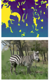
The resulting automated complexity metric (number of distinct mean-shift segmented regions) turns out to correlate quite well with human judgments of complexity, at least for images from the SAVOIAS visual complexity dataset. My filtering method successfully prevents redundant regions from being factored into an image’s complexity, as shown in the image below. The bottom shows the mean-shift segmentation of the image and the top shows redundant regions, which were filtered out (blue), and distinct regions (yellow), which are counted to yield the image’s complexity score:
For now, I will be using distinct number of mean-shift segmented regions as a metric to determine the groundtruth complexity of images from the COCO dataset, in order to train a text-based classifier to identify complex and non-complex COCO images from their captions. Professor Ordóñez-Román also mentioned that we might revisit the problem of choosing a better complexity metric in later weeks.
Next, I worked on calculating my complexity metric for all ~123,000 images from the COCO dataset (before, I had been working with just a small, 5,000-image subset). Professor Ordóñez-Román introduced me to a trick for parallelizing this computation so that it doesn’t take 4 days! Simply launch a script to process the images in multiple screens, and let it run in the background. In each screen, the script loops over and processes the images in random order (so as to avoid collisions), checking first if each image has already been processed. This cut down the compute time down to a few hours.
I’m now working on analyzing the resulting data and writing dataset and dataloader classes, so that the data is compatibly structured for loading into a machine learning model built with PyTorch. I also created pages to display the most and least complex validation set images.
Next week:
- Training BERT to classify images as complex/non-complex from their captions.