Week 3 (May 30 - June 3, 2022)
This week I reviewed several possible datasets which we could use to analyze visual complexity: Conceptual Captions 3M and 12M, LAION-400M, SAVOIAS, MS-COCO, and SBU. I recorded how images and captions for each of these datasets were collected to determine which would be most appropriate for my project.
One dilemma is that SAVOIAS is the only dataset of the above that includes annotations for visual complexity. However, SAVOIAS has no captions, so if we want to relate visual with linguistic complexity, we would have to collect captions. SAVOIAS is also very small (1420 images) compared to the other datasets (the next smallest, MS-COCO, has 328,000 images).
Although the other datasets have captions, they lack visual complexity annotations, so we have to come up with a metric that adequately captures visual complexity in order to use the non-complexity-annotated datasets. When the SAVOIAS authors compared their human-generated complexity annotations to several baseline visual complexity measurement algorithms, however, they found that none were especially robust across all 7 categories of images. It did occur to me that we might combine several of these metrics to get a better measure of visual complexity.
Additionally, Professor Ordóñez-Román pointed out that for the categories of SAVOIAS which we’re interested in (Objects, Scenes, Interiors), number of image regions (as measured by mean-shift segmentation) and a measure called feature congestion worked relatively well. Unfortunately, the SAVOIAS authors did not include p-values for their reported correlations of these metrics with the human-annotated visual complexity scores, or details of how these baseline metrics were computed in their paper (besides citations of the papers that explain how each metric is calculated).
So, my next steps this week were to recalculate the number of image regions and feature congestion for images in the Objects, Scenes, Interiors categories of SAVOIAS, and compute the Pearson correlation coefficient for those 2 automated measures of visual complexity with the human-annotated SAVOIAS scores, to see if any of these automated visual complexity measures reasonably capture human intuition about visual complexity. Professor Ordóñez-Román also suggested that I use DeepLabV3 for image segmentation to see if I get a better correlation than using mean-shift segmentation, which is a relatively old method. I also created pages to display the SAVOIAS images, sorted by visual complexity, so that we can inspect whether the SAVOIAS annotations make sense.
I also spent some time familiarizing myself with mean-shift segmentation and feature congestion.
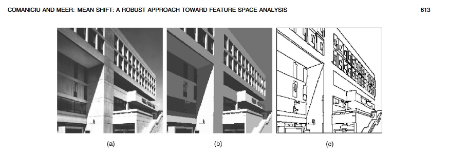
(Side note: mean-shift filtering has the cool artistic effect of making photos look like paintings/drawings. The example below is from Comaniciu and Meer, 2002.)
Originally, I was going to use OpenCV for mean-shift segmentation, but OpenCV is written in C++, and I could not get the Python bindings to generate for the specific function I needed. (As far as I could tell, this was because the function is part of the contrib/extra modules of OpenCV, not the main library). However, Professor Ordóñez-Román suggested an alternative Python function which I got to work this afternoon.
I started looking through the GitHub documentation for the implementation of the Feature Congestion metric, but it’s going to take me more time to parse through how to choose the correct parameters to calculate it.
Another metric of visual complexity we might use are the experimental results that vislang has run on some of the MS-COCO images. People are shown an image and asked to determine if certain objects (e.g., a bird) are present as quickly as possible. Presumably, a more complex image will make it harder for people to identify the presence/absence of a particular object, so the time they spend on the task can act as a proxy for image complexity.
In other news, I had periodontal surgery this week, which meant I had to take a few days off. My recovery is going well so far.
To-dos for next week:
- Finish computing number of regions and feature congestion metrics for Scenes, Objects, and Interiors categories of SAVOIAS, and compute correlations between each of these metrics with human-annotated SAVOIAS visual complexity scores.
References: Comaniciu, D., & Meer, P. (2002). Mean shift: A robust approach toward feature space analysis. IEEE Transactions on Pattern Analysis and Machine Intelligence, 24(5), 603–619. https://doi.org/10.1109/34.1000236